3D structure
The 3D Structure module builds a steel-frame building from grids and levels, loads it, analyzes it (second order, with the AISC 360-22 Direct Analysis Method by default) and turns every joint into a connection with its forces, plus plans of the structure with their details. Open it from New → 3D Structure, the start screen or Ctrl+K.
The screen#
The module uses the whole window. The top bar holds the N (back to the Nexum start screen), the model name (click to rename), the six steps 1 Model · 2 Define · 3 Loads · 4 Analysis · 5 Connections · 6 Plans (a ✓ replaces the number once the step is done), and undo, redo, save and close.
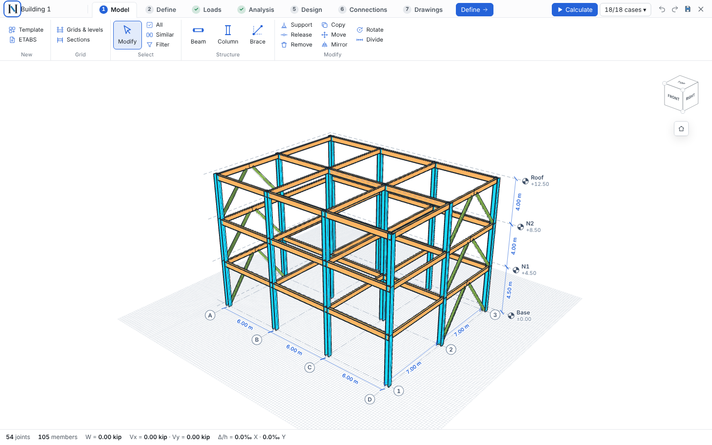
Below it, the ribbon of the open step: big buttons for what you use most, small stacked ones for the rest, and Next → on the right. Side panels appear only when needed: on the left in Define and Loads, or in Model when you open Grids & levels or Sections; on the right for what you selected and, with nothing selected, the analysis summary (step 4) or the connection list (step 5).
Model#
- Template: building, warehouse or mezzanine with bays, spans, levels and heights.
- Grids & levels: editable tables. Braces can be X, chevron, single diagonal or eccentric (EBF, with a link of length e). Insert an intermediate grid (A.1, 1.1) between two others: the rest keep their names, beams crossing it are split and keep their section, releases and loads. Insert a level below another (the story is split; other elevations don't move).
- Draw beams, columns and braces point to point with snapping to nodes and midpoints.
- Select with click, Shift+click, Shift+drag window, All, Same and Filter. With several members selected you can change their section and end releases, copy them to other levels, stop columns at a level (or leave a grid crossing empty), add loads or delete them.
Define#
Sections in the model (members, weight, steel; assign, replace everywhere, add from the AISC v15 database) and materials.
Materials are cards that say where every value comes from. Each material has a rule for E: steel (29 000 ksi), NTC concrete class 1 (limestone or basalt aggregate) or class 2, ACI 318 (4700√f′c MPa), k·√f′c, NTC masonry (800·fm for concrete block, 600·fm for clay) or a value you type. The card shows the substitution step by step and flags values out of range (for example E of masonry entered in kgf/m² instead of kgf/cm²). Imported ETABS materials keep their values and the rule is deduced from E.
Walls and slabs use shell properties: thick (with shear deformation), thin (Kirchhoff, shear stiffened ×100) or membrane (in-plane only). Stiffness modifiers f11, f22, f12, m11, m22, m12, v13 and v23 work as in ETABS. Walls can be any polygon and have openings; slabs with a shell property are meshed and carry their loads to the mesh.
Loads#
Pick the pattern (D, L, La, Ex, Ey, Wx, Wy), then: area loads per level, line loads (uniform or trapezoidal, full or partial length, gravity or X/Y), node loads (P, Fx, Fy, Mx, My, Mz) and rectangular load zones. Patterns sets the design wind pressure and the seismic load: static (coefficient c per direction, forces ∝ W·h applied at the center of mass) or response spectrum, edited in the Response spectrum window, which has the same parts as an ETABS response spectrum function and load case: the function (ASCE 7-16 from Ss, S1 and the site class — Fa and Fv from Tables 11.4-1 and 11.4-2, or your own where the table refers to §11.4.8 —, ASCE 7-22 with SDS, SD1 and TL, a parametric a0, c, Ta, Tb, r spectrum as in the CFE-93 manual and Mexican state codes, or a table of T–Sa points pasted from Excel, SASID or the USGS multi-period spectrum; "Convert to points" makes any function editable), the reduction (Ie, R, and Q with Q′(T) for the parametric one), the load case (CQC, SRSS or ABS modal combination, damping for the CQC, number of modes, scaling to the static base shear — 1.0 per ASCE 7-22 §12.9.1.4.1 — and accidental eccentricity) and the displacements (Cd and allowable drift). The large plot marks T0, Ts and TL (or Ta and Tb) and the period of every mode with more than 5 % of the mass; hover to read T, elastic Sa and design Sa. Below it: the modes table and, per direction, the modal, minimum and design base shear, the scale factor and the amplified drift against the allowable. The story forces (differences of the combined story shears) are applied as the seismic pattern, so they enter the combinations, the second-order analysis and the connections with sign. Accidental torsion (static and spectral; 5 % by default per ASCE 7-22 §12.8.4.2, the NTC requires 10 %) is applied as Mt = e·b·F per level, and every seismic combination is run with +e and −e (the "e" column of the combinations table changes it); Combinations is a spreadsheet of combinations generated from the selected code (NTC A/B, ASCE LRFD/ASD, NSR-10, E.090) that you can edit.
Analysis#
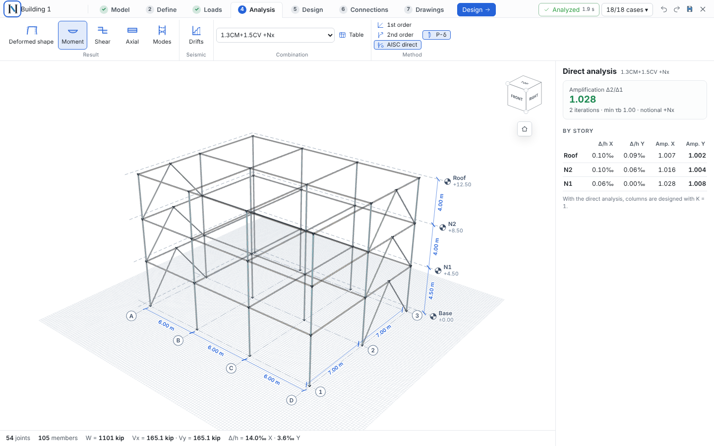
The analysis does not run on every edit: it runs in a background thread when you press Run (F5). The arrow next to it picks which combinations to compute (the envelope uses only those) and turns Auto on or off. While results are out of date the model is drawn in grey with a "Results out of date · F5" banner; geometry, loads and properties can be edited without waiting.
| Method | What it does |
|---|---|
| Direct AISC (default) | Second order with P-Δ and P-δ, 0.8·τb·EI and 0.8·EA, notional loads 0.002·Yi. Design columns with K = 1. |
| 2nd order | Second order with nominal stiffness and no notional loads |
| 1st order | Linear; combinations are the sum of patterns |
With the Direct Analysis Method every gravity-only combination is analyzed four times, with notional loads in +X, −X, +Y and −Y. Combinations with lateral loads get notional loads only if Δ2/Δ1 > 1.7. With nothing selected, the right panel shows the Δ2/Δ1 amplification (green up to 1.5, orange above, red if it does not converge), iterations, the smallest τb and a per-story table of drift and amplification. If a combination exceeds the critical load you get a red warning naming the node where stiffness is lost.
The second-order solver was verified against closed-form solutions (cantilever with axial and lateral load) and against
OpenSees (PDelta transformation with Newton) on the full building: differences below 0.03 %.
Modes#
Modes in the Analysis ribbon lists periods and effective modal mass in X and Y (cumulative, warning below 90 %); click a row to draw that mode shape. Eigen vectors find the lowest modes; Ritz vectors (Analysis → Modes) start from the load patterns and reach the participating mass with far fewer modes when walls have many local out-of-plane modes. Unchecking Modal skips it unless the seismic load is spectral.
Piers and spandrels: label walls as piers (P1, P2…) or spandrels (S1…) and the Analysis panel lists P, V2, M3 at
the top and bottom of each pier and V, M at each end of each spandrel, integrated from the shell forces at the cut. With a response spectrum it also shows the modal vs. static base shear, the scale
factor applied and, per story, the CQC drift and the equivalent story force. Periods and effective masses were verified
against OpenSees eigen (< 0.001 %).
Member design#
The Design step checks every beam, column and brace per AISC 360-16, with the same checks as the Member template (verified against the AISC Companion v15.1): tension, compression, flexure about both axes with lateral-torsional buckling, shear, torsion when present and the H1 interaction, along the whole member and for every strength combination. The 3D view colors each member by its governing ratio (light green < 50 %, green 50–80 %, dark green 80–95 %, orange up to 100 %, red when failing). Click a member to see the governing check and combination, change its section, the unbraced lengths (Lc x, Lc y, Lb of the top and bottom flanges), the service deflection of beams vs. L/240 and every check step by step. Lighten / Upsize to … proposes the lightest section of its series that passes with the current forces (then the model is reanalyzed); Resize the failing members does it for all of them. Table lists every member, sortable, filterable and ready to copy to Excel. Assumptions: K = 1 (allowed by the direct analysis method); members are braced at their ends and at every joint where another member frames in; with Slab bracing (on by default) the slab also braces the weak axis and the top flange of the beams along their full length.
For the selected member, Ends and connections sets each end Continuous (moment connection) or Pinned (shear connection) and reanalyzes; below each end, the connection detected at that joint opens its group in Connections. Member calculation report creates (or updates) an Element in the project with this member and the diagrams of every combination, with the same utilization. Report in the ribbon builds the calculation report of the whole structure (summary, geometry, sections with maximum demands, loads, seismic and modes, combinations, reactions, drifts and every member's design), ready to print or save as PDF.
Drifts#
Analysis → Drifts (or click Δ/h in the status bar): per story and direction, the elastic drift Δe (seismic plus accidental torsion, governing sign), the design drift Δ = Cd·Δe/Ie against the limit, the torsional irregularity δmax/δavg at both ends of the plan (type 1a > 1.2, 1b > 1.4, with Ax), the stability coefficient θ against θmax (ASCE 7-22 Eq. 12.8-16/17) and the participating modal mass, with a drift-per-level chart.
View, windows and modeling operations#
Two fixed groups sit at the right of the ribbon on every tab:
- View: 3D · Plan · Elevation X · Elevation Y (Alt+1 … Alt+4), Solid · Sticks (B toggles: the analytical joint-to-joint model, like the ETABS line view), By section and Section box with To selection, All and Cut at grid…. Grids carry their bubbles and levels their heads, as in Revit.
- Windows opens floating windows you drag by their title bar anywhere on the canvas; several at once, collapse them
(double click or _) and close them (×). The ones you have not moved arrange themselves without overlapping.
- Properties: the selection (section, ends, loads, copy to levels) in a window; closed, it docks on the right.
- Visibility: grids, levels, dimensions, joint numbers, member labels, display (solid or sticks) and color.
- Modeling: Copy (ΔX, ΔY, ΔZ in m and number of copies = array; one-bay and one-story buttons), Move, Mirror (plane X = c or Y = c, on a grid line or at a distance, with or without a copy), Rotate (about a vertical axis, typed center or the selection's, with copies) and Divide (equal parts). Applies to the selection; undo with Ctrl+Z. New items are free joints and drawn members: a joint that falls on another is that one, and a member that already exists between the same two joints is not duplicated. Each copy keeps section, steel, rotation, releases, its loads and the supports of its base joints.
- Options: snap to joints, midpoints and grid intersections at every level (creates the joint when used); chain beams and braces; pinned or continuous beams when drawing; beam, column and brace sections when drawing.
- Views (browser, like Revit's): 3D, a plan per level, an elevation per grid line and saved views with their direction and section box (stored in the project).
Importing an ETABS model#
Model → New → ETABS (also on the start screen and Ctrl+K): pick the .e2k (File → Export → ETABS .e2k Text File; a
.$et also works). It replaces the model (can be undone) and shows a report of what came across, what was adjusted and
what could not be imported. Joints and frames keep their ETABS names (point@story).
Imported: units (also with decimal commas), stories, grids, diaphragms, materials, sections (AISC catalog, metric names, user I and box shapes that are designed, pipes, rectangles and circles of steel or concrete, general sections, angles, channels and tees, auto select lists with their starting section, nonprismatic with the start section, section and member modifiers), columns, beams and braces with rotation and 6-DOF releases, supports (springs as rigid supports), joint and line masses, active DOF, floors as load panels (one- or two-way, with self weight), load patterns, joint, frame (uniform, trapezoidal and point; gravity, global, local or projected) and area loads (also uniform load sets), the response spectrum (user or ASCE 7 function) with its case and number of modes, the mass source, auto static seismic (ASCE 7 or user coefficient) and load combinations (linear add, envelopes and nested; spectral ones with + and −).
Not imported (the report says so): walls and other shell areas, frame moment loads, end offsets and rigid zones, auto wind (the pattern has no pressure) and nonlinear or time-history cases. Verified against ETABS verification examples 6 and 7 (eigenvalues within 0.0004 %; periods, roof displacement and column forces within 0.005 %).
Element information#
Right-click any member, node, wall or slab for its information sheet, laid out like ETABS' Object information: the object ID row, then Geometry, Assignments and Loads tabs. Rows expand (end releases, modifiers), modified values are marked, and section, releases, wall property, pier/spandrel label and node restraints can be edited in place. The ↗ link on a material, section, shell property or load opens the window where it is defined.
Connections and plans#
Equal joints form a group; each group gets one connection with one load case per strength combination (the joint that works hardest in each). Create connections adds them to the project or updates their loads without touching their design. Plans shows a plan per level and an elevation per grid with detail bubbles, then the detail sheets; export to PDF or a single DXF.
Not yet#
Seismic capacity design per AISC 341 in the member design, amplification of accidental torsion (Ax), time-history analysis, code wind pressure coefficients, shear deformation and rigid end offsets, nonlinear walls and wall design per ACI 318 ch. 11 and 18.